This notebook is available on GitHub.
Interactive online version:
![]()
Test computational scaling
Here we give an example of how to measure the training computation time as a function of training iteration and number of dimensions.
[1]:
import alabi
from alabi.core import SurrogateModel
from alabi import benchmarks as bm
import numpy as np
import matplotlib.pyplot as plt
from functools import partial
from scipy.stats import multivariate_normal
Define common settings for all tests
[2]:
ncore = 1                       # we'll run one active learning chain on one core
ntrain = 100                    # number of initial training samples
savedir = "results/scaling"     # directory to save results

gp_kwargs = {"kernel": "ExpSquaredKernel",
             "fit_amp": True,
             "fit_mean": True,
             "fit_white_noise": False,
             "white_noise": -12,
             "gp_opt_method": "l-bfgs-b",
             "gp_scale_rng": [-2,2],
             "optimizer_kwargs": {"max_iter": 50, "xatol": 1e-3, "fatol": 1e-2, "adaptive": True}}

al_kwargs = {"algorithm": "bape",
             "gp_opt_freq": 20,
             "obj_opt_method": "nelder-mead",
             "nopt": 1,
             "optimizer_kwargs": {"max_iter": 50, "xatol": 1e-3, "fatol": 1e-2, "adaptive": True}}
Define a general function that trains alabi on an N-dimensional Gaussian for max_iter iterations
[3]:
def run_alabi(ndim, max_iter=100, savedir="results/scaling"):

    path = f"{savedir}/multivariate_normal_{ndim}d/"

    # Define the multivariate normal likelihood function
    mean = np.zeros(ndim)
    cov = bm.random_gaussian_covariance(ndim)
    lnlike = partial(multivariate_normal.logpdf, mean=mean, cov=cov)

    # Train surrogate model
    sm = SurrogateModel(lnlike_fn=lnlike,
                        bounds=[(-3., 3.) for _ in range(ndim)],
                        savedir=path,
                        cache=True,
                        verbose=True,
                        ncore=ncore)

    # save the true mean and covariance to a file
    np.savez(f"{path}gaussian_mean_cov.npz", mean=mean, cov=cov)

    # Initialize surrogate model
    if ndim >= 40:
        sm.init_samples(ntrain=ntrain, sampler="uniform")
    else:
        sm.init_samples(ntrain=ntrain, sampler="sobol")

    sm.init_gp(**gp_kwargs)
    sm.active_train(niter=max_iter, **al_kwargs)
    sm.plot(plots=["gp_all"])
For a quick test, we’ll just run alabi for a 5-dimensional gaussian and measure the amount of computational overhead alabi takes to train the surrogate model. To test more dimensions add them to the dimensions array, or to test for more iterations increase max_iter.
[4]:
dimensions = [5]
# dimensions = [10, 20, 30]

# Test the scaling of ALABI with dimensionality
for ndim in dimensions:
    run_alabi(ndim, max_iter=200, savedir=savedir)
Initialized GP with squared exponential kernel.
Successfully initialized GP on attempt 1

Optimizing GP hyperparameters using 5-fold cross-validation...
Evaluating 100 hyperparameter candidates using 5-fold CV...
Running 200 active learning iterations using bape...
8%|▊ | 17/200 [00:00<00:02, 79.35it/s]
Optimizing GP hyperparameters using 5-fold cross-validation...
Evaluating 100 hyperparameter candidates using 5-fold CV...
16%|█▋ | 33/200 [00:00<00:04, 35.49it/s]
Train MSE: 5.290769548379788e-16

Optimizing GP hyperparameters using 5-fold cross-validation...
Evaluating 100 hyperparameter candidates using 5-fold CV...
24%|██▍ | 49/200 [00:01<00:05, 29.95it/s]
Train MSE: 2.8140615805435077e-16
29%|██▉ | 58/200 [00:01<00:03, 38.40it/s]
Optimizing GP hyperparameters using 5-fold cross-validation...
Evaluating 100 hyperparameter candidates using 5-fold CV...
36%|███▋ | 73/200 [00:02<00:04, 28.77it/s]
Train MSE: 4.740593184211731e-16

Optimizing GP hyperparameters using 5-fold cross-validation...
Evaluating 100 hyperparameter candidates using 5-fold CV...
44%|████▎ | 87/200 [00:03<00:04, 24.17it/s]
Train MSE: 1.5158058487886292e-15
47%|████▋ | 94/200 [00:03<00:03, 29.82it/s]
Optimizing GP hyperparameters using 5-fold cross-validation...
Evaluating 100 hyperparameter candidates using 5-fold CV...
54%|█████▍ | 108/200 [00:04<00:03, 24.03it/s]
Train MSE: 5.561937160794517e-15
57%|█████▊ | 115/200 [00:04<00:02, 29.48it/s]
Optimizing GP hyperparameters using 5-fold cross-validation...
Evaluating 100 hyperparameter candidates using 5-fold CV...
64%|██████▍ | 128/200 [00:05<00:03, 21.95it/s]
Train MSE: 1.3563998408462552e-14
68%|██████▊ | 135/200 [00:05<00:02, 27.36it/s]
Optimizing GP hyperparameters using 5-fold cross-validation...
Evaluating 100 hyperparameter candidates using 5-fold CV...
74%|███████▎ | 147/200 [00:06<00:02, 18.96it/s]
Train MSE: 3.814731814602212e-12
80%|███████▉ | 159/200 [00:06<00:01, 27.91it/s]
Optimizing GP hyperparameters using 5-fold cross-validation...
Evaluating 100 hyperparameter candidates using 5-fold CV...
84%|████████▍ | 168/200 [00:07<00:02, 14.01it/s]
Train MSE: 2.661067977783123e-10
90%|████████▉ | 179/200 [00:07<00:00, 22.16it/s]
Optimizing GP hyperparameters using 5-fold cross-validation...
Evaluating 100 hyperparameter candidates using 5-fold CV...
92%|█████████▏| 184/200 [00:09<00:01, 9.85it/s]
Train MSE: 2.6148026975461192e-09
98%|█████████▊| 195/200 [00:09<00:00, 16.86it/s]
Optimizing GP hyperparameters using 5-fold cross-validation...
Evaluating 100 hyperparameter candidates using 5-fold CV...
100%|██████████| 200/200 [00:10<00:00, 18.99it/s]
Train MSE: 2.0152473853508697e-07
Caching model to results/scaling/multivariate_normal_5d/surrogate_model...
Plotting the gp mean squared error with 0 test samples...
Saving to results/scaling/multivariate_normal_5d//gp_mse_vs_iteration.png
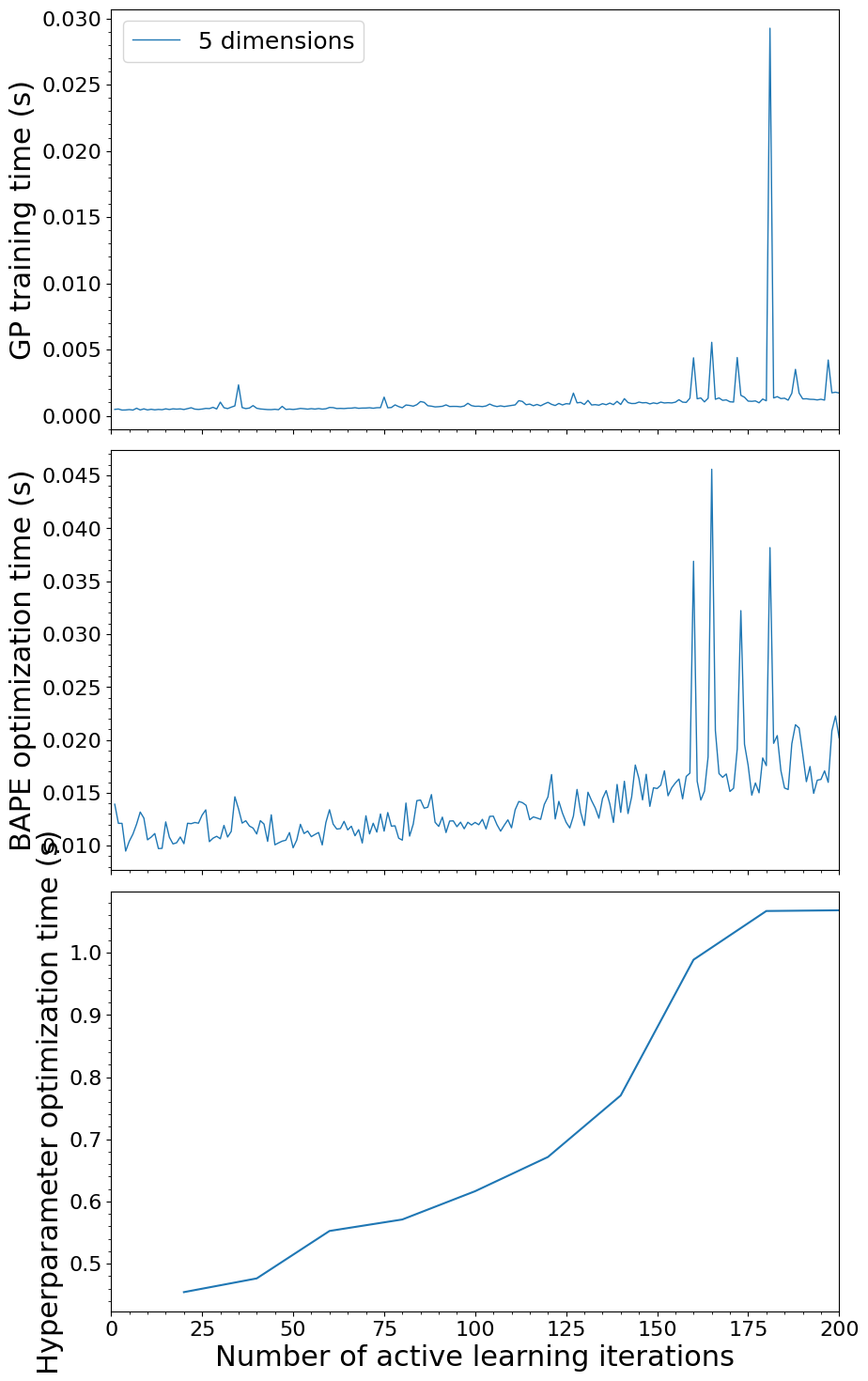
Get the recorded train time for each step of alabi’s training process.
[5]:
train_time = []
opt_time = []
test_mse = []
hp_opt_time = []
hp_opt_iter = []

for ndim in dimensions[::-1]: # Reverse order for plotting
    path = f"{savedir}/multivariate_normal_{ndim}d/"
    sm = alabi.load_model_cache(path)
    train_time.append(sm.training_results['gp_train_time'])
    opt_time.append(sm.training_results['obj_fn_opt_time'])
    test_mse.append(sm.training_results['test_mse'])
    hp_opt_time.append(sm.training_results['gp_hyperparam_opt_time'])
    hp_opt_iter.append(sm.training_results['gp_hyperparameter_opt_iteration'])
iterations = sm.training_results['iteration']

train_time = np.array(train_time)
opt_time = np.array(opt_time)
test_mse = np.array(test_mse)
hp_opt_time = np.array(hp_opt_time)
hp_opt_iter = np.array(hp_opt_iter)

cum_time = np.sum(train_time, axis=1) + np.sum(opt_time, axis=1) + np.sum(hp_opt_time, axis=1)
[6]:
logy = False

fig, (ax1, ax2, ax3) = plt.subplots(3, 1, figsize=(10, 18), sharex=True)
plt.subplots_adjust(hspace=0.05)

# Top panel - Training time
for ii, ndim in enumerate(dimensions):
    ax1.plot(iterations, train_time[ii], label=f"{dimensions[ii]} dimensions", linewidth=1)
ax1.set_ylabel("GP training time (s)", fontsize=22)
ax1.legend(loc="upper left", fontsize=18)
ax1.minorticks_on()

# Middle panel - Optimization time
for ii, ndim in enumerate(dimensions):
    ax2.plot(iterations, opt_time[ii], linewidth=1)
ax2.set_ylabel("BAPE optimization time (s)", fontsize=22)
ax2.minorticks_on()

# # Bottom panel - Total time
for ii, ndim in enumerate(dimensions):
    ax3.plot(hp_opt_iter[ii], hp_opt_time[ii][1:], linewidth=1.5)
ax3.set_xlabel("Number of active learning iterations", fontsize=22)
ax3.set_ylabel("Hyperparameter optimization time (s)", fontsize=22)
ax3.minorticks_on()

if logy:
    ax1.set_yscale("log")
    ax2.set_yscale("log")
    # ax3.set_yscale("log")
ax1.set_xlim(0, iterations[-1])

plt.savefig(f"{savedir}/multivariate_normal_training_time.png", bbox_inches='tight', dpi=800)
plt.show()
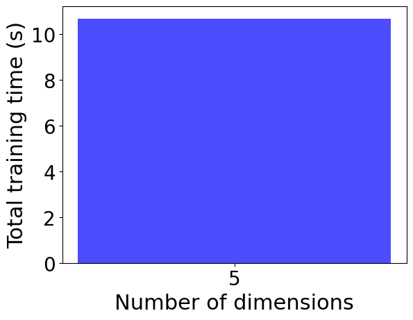
Plot the cummulative training time as a bar chart for each dimension.
[7]:
plt.bar(dimensions, cum_time, width=1, color='blue', alpha=0.7)
plt.xlabel("Number of dimensions", fontsize=22)
plt.ylabel("Total training time (s)", fontsize=22)
plt.xticks(dimensions, fontsize=20)
plt.yticks(fontsize=20)
plt.savefig(f"{savedir}/multivariate_normal_total_training_time.png", bbox_inches='tight', dpi=600)
plt.show()