This notebook is available on GitHub.
Interactive online version:
![]()
Bayesian Optimization
In addition to inference problems, alabi can also be used for optimizing computationally expensive functions. This notebook demonstrates how to use alabi for Bayesian optimization on a 1D multimodal function using the Jones (Expected Improvement) active learning algorithm.
Import Libraries
First, let’s import the necessary libraries:
[2]:
import numpy as np
import matplotlib.pyplot as plt
from alabi.core import SurrogateModel
import warnings
warnings.filterwarnings('ignore')

from matplotlib import rcParams
# rcParams['font.family'] = 'serif'
# rcParams['text.usetex'] = True
Define the Multimodal Test Function
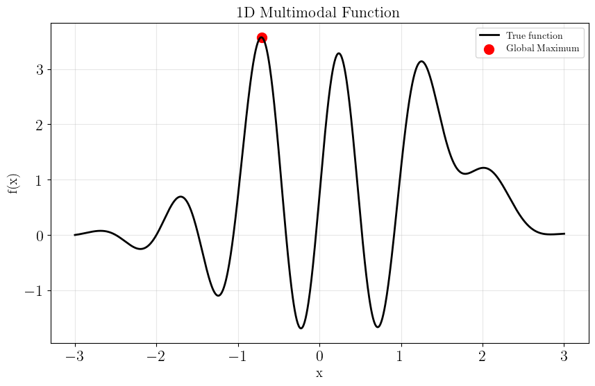
We’ll use a 1D multimodal function with multiple local maxima. This function combines a sine wave with a Gaussian peak to create an interesting optimization landscape:
[3]:
def multimodal_function(theta):
    """
    A 1D multimodal function with multiple peaks.
    Global maximum is around x=1.5
    """
    x = theta[0] if hasattr(theta, '__len__') else theta

    # Combine sine wave with Gaussian peaks
    f1 = 3 * np.sin(2 * np.pi * x) * np.exp(-0.5 * x**2)
    f2 = 2 * np.exp(-2 * (x - 1.5)**2)
    f3 = 1.5 * np.exp(-3 * (x + 0.5)**2)

    return f1 + f2 + f3

def plot_function(x_plot, y_plot):
    fig = plt.figure(figsize=(10, 6))
    plt.plot(x_plot, y_plot, 'k-', linewidth=2, label='True function')
    plt.scatter(x_plot[np.argmax(y_plot)], np.max(y_plot), color='red', s=100, label='Global Maximum')
    plt.xlabel('x', fontsize=14)
    plt.ylabel('f(x)', fontsize=14)
    plt.title('1D Multimodal Function', fontsize=16)
    plt.grid(True, alpha=0.3)
    plt.legend()

    print(f"True global maximum at x={x_plot[np.argmax(y_plot)]:.3f} with f(x)={np.max(y_plot):.3f}")

    return fig
[4]:
# Visualize the function
x_plot = np.linspace(-3, 3, 1000)
y_plot = [multimodal_function(x) for x in x_plot]

fig = plot_function(x_plot, y_plot)
True global maximum at x=-0.712 with f(x)=3.573
Set up the Surrogate Model
Now we’ll create a SurrogateModel using alabi. For optimization, we want to maximize the function, but alabi works with log-likelihood functions (which we typically want to maximize). So we’ll use our function directly as the “log-likelihood”.
[5]:
# Define bounds for the parameter space
bounds = [(-3.0, 3.0)]

# Create the surrogate model
sm = SurrogateModel(
    lnlike_fn=multimodal_function,
    bounds=bounds,
    param_names=['x'],
    cache=False,  # Disable caching for this demo
    verbose=True,
)
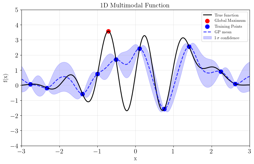
Initialize Training Set
Start with a small set of initial training points. First we’ll try training alabi with the default GP settings (using the squared exponential kernel and log-length scales ranging [-2,2]).
[6]:
# Initialize with a few random points
sm.init_samples(ntrain=10, sampler='lhs')

gp_kwargs = {"kernel": "ExpSquaredKernel",
             "fit_amp": True,
             "fit_mean": True,
             "fit_white_noise": False,
             "white_noise": -12,
             "gp_opt_method": "l-bfgs-b",
             "gp_scale_rng": [-1,1],
             "optimizer_kwargs": {"max_iter": 50},
             "overwrite": True}

sm.init_gp(**gp_kwargs)
Initialized GP with squared exponential kernel.
Successfully initialized GP on attempt 1

Optimizing GP hyperparameters using 5-fold cross-validation...
Evaluating 100 hyperparameter candidates using 5-fold CV...
[7]:
xpred = np.linspace(-3, 3, 200).reshape(-1,1)
ypred, yvar = sm.surrogate_log_likelihood(xpred, return_var=True)
ystd = np.sqrt(yvar)

fig = plot_function(x_plot, y_plot)
plt.scatter(sm.theta_train[:sm.ninit_train].flatten(), sm.y_train[:sm.ninit_train], color='blue', s=100, label='Training Points')
plt.plot(xpred.flatten(), ypred, 'b--', linewidth=2, label='GP mean', alpha=0.8)
plt.fill_between(xpred.flatten(), ypred - ystd, ypred + ystd,
                 color='b', alpha=0.2, label=f'$1\,\sigma$ confidence')
plt.xlim(*sm.bounds)
plt.ylim(-4,5)
plt.legend()
plt.show()
True global maximum at x=-0.712 with f(x)=3.573
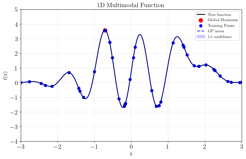
Run Bayesian Optimization with Jones Algorithm
The Jones algorithm (Expected Improvement) is designed for optimization. It balances exploration (uncertainty) with exploitation (improving the current best).
[8]:
# Run active learning with Jones algorithm
niter = 30
sm.active_train(
    niter=niter,
    algorithm="jones",  # Use Jones (Expected Improvement) algorithm
    gp_opt_freq=5,     # Re-optimize GP hyperparameters every 5 iterations
)
Running 30 active learning iterations using jones...
0%| | 0/30 [00:00<?, ?it/s]
Optimizing GP hyperparameters using 5-fold cross-validation...
Evaluating 100 hyperparameter candidates using 5-fold CV...
17%|█▋ | 5/30 [00:00<00:02, 8.46it/s]
Train MSE: 3.183613129229024e-10

Optimizing GP hyperparameters using 5-fold cross-validation...
Evaluating 100 hyperparameter candidates using 5-fold CV...
33%|███▎ | 10/30 [00:01<00:02, 8.96it/s]
Train MSE: 2.202458513687688e-08

Optimizing GP hyperparameters using 5-fold cross-validation...
Evaluating 100 hyperparameter candidates using 5-fold CV...
50%|█████ | 15/30 [00:01<00:01, 9.18it/s]
Train MSE: 5.730703548005629e-10

Optimizing GP hyperparameters using 5-fold cross-validation...
Evaluating 100 hyperparameter candidates using 5-fold CV...
67%|██████▋ | 20/30 [00:02<00:01, 9.20it/s]
Train MSE: 5.327356039977324e-10

Optimizing GP hyperparameters using 5-fold cross-validation...
Evaluating 100 hyperparameter candidates using 5-fold CV...
83%|████████▎ | 25/30 [00:02<00:00, 9.27it/s]
Train MSE: 1.1479125404715901e-09

Optimizing GP hyperparameters using 5-fold cross-validation...
Evaluating 100 hyperparameter candidates using 5-fold CV...
100%|██████████| 30/30 [00:03<00:00, 9.18it/s]
Train MSE: 6.8732024410845975e-09
[9]:
xpred = np.linspace(-3, 3, 200).reshape(-1,1)
ypred, yvar = sm.surrogate_log_likelihood(xpred, return_var=True)
ystd = np.sqrt(yvar)

fig = plot_function(x_plot, y_plot)
plt.scatter(sm.theta(), sm.y(), color='blue', s=50, label='Training Points')
plt.plot(xpred.flatten(), ypred, 'b--', linewidth=2, label='GP mean', alpha=0.8)
plt.fill_between(xpred.flatten(), ypred - ystd, ypred + ystd,
                 color='b', alpha=0.2, label=f'$1\,\sigma$ confidence')
plt.xlim(*sm.bounds)
plt.ylim(-4,5)
plt.legend()
plt.show()
True global maximum at x=-0.712 with f(x)=3.573
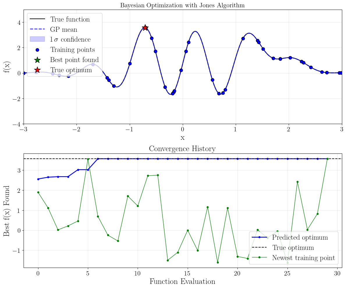
Visualize the Optimization Process
Let’s create a visualization showing the true function, the GP surrogate model, and the points selected by the Jones algorithm.
[10]:
# Get GP predictions over the domain
xpred = np.linspace(-3, 3, 200).reshape(-1,1)

x_best_iter, y_best_iter = [], []
for it in range(sm.nactive):
    ypred, yvar = sm.surrogate_log_likelihood(xpred, iter=it, return_var=True)
    ystd = np.sqrt(yvar)

    best_idx = np.argmax(ypred)
    best_x = xpred[best_idx]
    best_f = ypred[best_idx]

    x_best_iter.append(best_x)
    y_best_iter.append(best_f)

true_optimum_idx = np.argmax(y_plot)
true_optimum_x = x_plot[true_optimum_idx]
true_optimum_f = y_plot[true_optimum_idx]
[11]:
# Final iteration prediction
ypred, yvar = sm.surrogate_log_likelihood(xpred, iter=-1, return_var=True)
ystd = np.sqrt(yvar)

plt.figure(figsize=(12,10))

# Plot true function
plt.subplot(2, 1, 1)
plt.plot(x_plot, y_plot, 'k-', linewidth=2, label='True function', alpha=0.8)

# Plot GP mean and uncertainty
plt.plot(xpred.flatten(), ypred, 'b--', linewidth=2, label='GP mean', alpha=0.8)
plt.fill_between(xpred.flatten(), ypred - ystd, ypred + ystd,
                 color='b', alpha=0.2, label=f'$1\,\sigma$ confidence')

# Plot training points
plt.scatter(sm.theta(), sm.y(),
           c='b', s=60, zorder=5, label='Training points', edgecolor='black')

# Highlight the best point
plt.scatter(best_x, best_f, c='green', s=250, marker='*',
           zorder=6, label='Best point found', edgecolor='black')

# Highlight true optimum
plt.scatter(true_optimum_x, true_optimum_f, c='red', s=250, marker='*',
           zorder=6, label='True optimum', edgecolor='black')

plt.xlabel('x', fontsize=20)
plt.ylabel('f(x)', fontsize=20)
plt.xlim(*sm.bounds)
plt.ylim(-4,5)
plt.title('Bayesian Optimization with Jones Algorithm', fontsize=16)
plt.legend(loc='upper left', fontsize=18)
plt.grid(True, alpha=0.3)

# Plot convergence history
plt.subplot(2, 1, 2)
plt.plot(range(len(y_best_iter)), y_best_iter, 'b-o', linewidth=2, markersize=4, label="Predicted optimum")
plt.axhline(y=true_optimum_f, color='k', linestyle='--', label='True optimum')
plt.plot(range(sm.nactive), sm.y()[sm.ninit_train:], "g-o", linewidth=1, markersize=4, label="Newest training point")
plt.xlabel('Function Evaluation', fontsize=20)
plt.ylabel('Best f(x) Found', fontsize=20)
plt.title('Convergence History', fontsize=20)
plt.legend(loc="lower right", fontsize=18)
plt.grid(True, alpha=0.3)

plt.tight_layout()
plt.show()
Summary
This example demonstrates how to use alabi for Bayesian optimization:
Problem Setup: We defined a 1D multimodal function with multiple local maxima
Surrogate Model: Created a
SurrogateModelwith the function and parameter boundsInitialization: Started with a small set of random training points
Optimization: Used the Jones algorithm (Expected Improvement) to iteratively select new points
Results: The algorithm successfully found the global maximum with high accuracy
The Jones algorithm is particularly effective for optimization because it:
Exploits known good regions (high function values)
Explores uncertain regions (high GP variance)
Balances these two objectives through the Expected Improvement criterion
This approach is much more efficient than random search or grid search, especially for expensive function evaluations.
Things to try next:
Different kernel functions (
ExpSquaredKernel,Matern32Kernel,Matern52Kernel)Increase the number of training samples
Run multiple trials for each setting to test how robust the training is to random sampling