This notebook is available on GitHub.
Interactive online version:
![]()
Installation + Quickstart
To install alabi, clone it from the git repo:
git clone https://github.com/jbirky/alabi
cd alabi
python setup.py install
Step 1
Import python modules:
[1]:
import numpy as np
import matplotlib.pyplot as plt

from alabi.core import SurrogateModel

from matplotlib import rcParams
# rcParams['font.family'] = 'serif'
# rcParams['text.usetex'] = True

random_state = 7
np.random.seed(random_state)
Step 2
Define the test function and the bounds for the input space. For example:
[2]:
def test1d_fn(x):
    return np.sin(5 * x) * (1 - np.tanh(x**2))

bounds = [(-1, 1)]
Step 3
Initialize the surrogate model, specifying the function to train on, the bounds of the input space, and directory where the results will be saved:
[3]:
sm = SurrogateModel(lnlike_fn=test1d_fn, bounds=bounds, savedir=f"results/test1d", random_state=random_state)
Step 4
Initialize the gaussian process surrogate model by specifying a kernel. In this example we’ll use a squared exponential kernel:
$ k(x, x’) = \sigma_f^2 \exp\left`(-:nbsphinx-math:frac{(x - x’)^2}{2ell^2}`:nbsphinx-math:right) $
where $ k(x, x’) $ is the kernel function, $ \sigma_f^2 $ is the amplitude hyperparameter, $ :nbsphinx-math:`ell `$ is the length scale hyperparameter, and $ x $ and $ x’ $ are input points.
[4]:
sm.init_samples(ntrain=10)
sm.init_gp(kernel="ExpSquaredKernel", fit_amp=True, fit_mean=True, hyperopt_method="ml", overwrite=True)
Initialized GP with squared exponential kernel.
Successfully initialized GP on attempt 1
Optimizing GP: 100%|██████████| 3/3 [00:00<00:00, 54.26it/s]
Initial -logL:   0.5847 |        Regularization: 1.6234 |        Total: 2.2081
Final -logL:     -8.6579 |       Regularization: 1.3110 |        Total: -7.3469
13 iterations | Success: True | Message: CONVERGENCE: RELATIVE REDUCTION OF F <= FACTR*EPSMCH
Step 5
Improve the surrogate model fit by iteratively selecting new training points using active learning:
[5]:
sm.active_train(niter=30, algorithm="bape", gp_opt_freq=10)
Running 30 active learning iterations using bape...
Optimizing GP: 100%|██████████| 3/3 [00:00<00:00, 53.97it/s]
 33%|███▎      | 10/30 [00:00<00:00, 72.83it/s]
Initial -logL:   -57.3958 |      Regularization: 1.3110 |        Total: -56.0848
Final -logL:     -59.0394 |      Regularization: 1.3352 |        Total: -57.7042
18 iterations | Success: True | Message: CONVERGENCE: RELATIVE REDUCTION OF F <= FACTR*EPSMCH

Train MSE: 9.298666599099183e-10
Optimizing GP: 100%|██████████| 3/3 [00:00<00:00, 60.86it/s]
 67%|██████▋   | 20/30 [00:00<00:00, 75.69it/s]
Initial -logL:   -121.3295 |     Regularization: 1.3352 |        Total: -119.9943
Final -logL:     -121.3499 |     Regularization: 1.3367 |        Total: -120.0132
17 iterations | Success: True | Message: CONVERGENCE: RELATIVE REDUCTION OF F <= FACTR*EPSMCH

Train MSE: 2.79227309296412e-09
Optimizing GP: 100%|██████████| 3/3 [00:00<00:00,  4.29it/s]
100%|██████████| 30/30 [00:02<00:00, 13.53it/s]
Initial -logL:   -185.4210 |     Regularization: 1.3367 |        Total: -184.0843
Final -logL:     -185.4270 |     Regularization: 1.3376 |        Total: -184.0893
6 iterations | Success: True | Message: CONVERGENCE: RELATIVE REDUCTION OF F <= FACTR*EPSMCH

Train MSE: 2.5884057559963692e-09
Caching model to results/test1d/surrogate_model...
Step 6
Run Markov Chain Monte Carlo (MCMC) sampler using either the emcee package:
[6]:
sm.run_emcee(nwalkers=4, nsteps=int(5e4))
Initializing emcee with self.surrogate_log_likelihood surrogate model as likelihood.
No prior_fn specified. Defaulting to uniform prior with bounds [[-1  1]]
Running emcee with 4 walkers for 50000 steps on 1 cores...

Run 1: Need 10000 more samples...
==================================================
100%|██████████| 50000/50000 [00:51<00:00, 973.36it/s]
burn-in estimate: 118
thin estimate: 29

Run 1 complete: 6880 samples
Total accumulated samples: 6880

Run 2: Need 3120 more samples...
==================================================
100%|██████████| 50000/50000 [00:50<00:00, 981.16it/s]
burn-in estimate: 105
thin estimate: 26

Run 2 complete: 7676 samples
Total accumulated samples: 14556

Combined 2 runs into 14556 total samples
Total samples: 14556
Mean acceptance fraction: 0.694
Mean autocorrelation time: 52.681 steps
Caching model to results/test1d/surrogate_model...
Saving final emcee samples to results/test1d/emcee_samples_final_surrogate_iter_30.npz ...
[7]:
sm.run_dynesty()
Initializing dynesty with self.surrogate_log_likelihood surrogate model as likelihood.
Initialized dynesty DynamicNestedSampler.
Running dynesty with 50 live points on 1 cores...

Run 1: Need 10000 more samples...
==================================================
10103it [00:09, 1057.98it/s, batch: 78 | bound: 0 | nc: 1 | ncall: 22538 | eff(%): 44.827 | loglstar: -inf < 0.909 < 0.295 | logz: 0.127 +/- 0.022 | stop: 0.999]
Run 1 complete: 10103 samples, logZ = 0.127
Total accumulated samples: 10103
Caching model to results/test1d/surrogate_model...
Saved dynesty samples to results/test1d/dynesty_samples_final_surrogate_iter_30.npz
[8]:
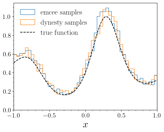
xgrid = np.linspace(bounds[0][0], bounds[0][1], 100)
ygrid = np.exp(test1d_fn(xgrid))

plt.hist(sm.emcee_samples.T[0], bins=50, histtype='step', density=True, label="emcee samples")
plt.hist(sm.dynesty_samples.T[0], bins=50, histtype='step', density=True, label="dynesty samples")
plt.plot(xgrid, ygrid/max(ygrid), label="true function", color="k", linestyle="--")
plt.xlabel("$x$", fontsize=25)
plt.xlim(*bounds)
plt.legend(loc="upper left", fontsize=18, frameon=False)
plt.minorticks_on()
plt.show()
[ ]: