This notebook is available on GitHub.
Interactive online version:
![]()
GP Training
This notebook demonstrates how to train a Gaussian process surrogate model using alabi and visualize the results.
[1]:
%matplotlib inline
import numpy as np
from alabi import SurrogateModel

from matplotlib import rcParams
# rcParams['font.family'] = 'serif'
# rcParams['text.usetex'] = True
Define a Test Problem: Rosenbrock Function
We’ll use the 2D Rosenbrock function as our test case. This is a common benchmark function for optimization and sampling algorithms.
[2]:
from scipy.optimize import rosen

def rosenbrock_fn(x):
    return -rosen(x)/100.0

bounds = [(-5,5), (-5,5)]
param_names = ['x1', 'x2']
Create and Train Surrogate Model
First, we’ll create a Gaussian Process surrogate model and train it using active learning.
[3]:
# Initialize the surrogate model
sm = SurrogateModel(
    lnlike_fn=rosenbrock_fn,
    bounds=bounds,
    savedir="results/rosenbrock_2d",
    cache=True,
    verbose=True,
    ncore=1
)

# Compute initial training samples (parallelized if ncore > 1)
sm.init_samples(ntrain=100, ntest=1000, sampler="lhs")
[4]:
# Initialize the Gaussian Process with specified hyperparameters
gp_kwargs = {"kernel": "ExpSquaredKernel",
             "fit_amp": True,
             "fit_mean": True,
             "fit_white_noise": False,
             "white_noise": -12,
             "gp_opt_method": "l-bfgs-b",
             "gp_scale_rng": [-2,2],
             "optimizer_kwargs": {"max_iter": 50}}

sm.init_gp(**gp_kwargs)
Initialized GP with squared exponential kernel.
Successfully initialized GP on attempt 1

Optimizing GP hyperparameters using 5-fold cross-validation...
Evaluating 100 hyperparameter candidates using 5-fold CV...
[4]:
np.float64(0.32818955109651066)
[5]:
al_kwargs={"algorithm": "bape",
           "gp_opt_freq": 20,
           "obj_opt_method": "nelder-mead",
           "use_grad_opt": True,
           "nopt": 1,
           "optimizer_kwargs": {"max_iter": 50, "xatol": 1e-3, "fatol": 1e-2, "adaptive": True}}

sm.active_train(niter=100, **al_kwargs)
Running 100 active learning iterations using bape...
18%|█▊ | 18/100 [00:00<00:01, 79.65it/s]
Optimizing GP hyperparameters using 5-fold cross-validation...
Evaluating 100 hyperparameter candidates using 5-fold CV...
34%|███▍ | 34/100 [00:01<00:02, 30.14it/s]
Train MSE: 0.08615299445103249
Test MSE: 0.22178853386779387

Optimizing GP hyperparameters using 5-fold cross-validation...
Evaluating 100 hyperparameter candidates using 5-fold CV...
47%|████▋ | 47/100 [00:01<00:02, 21.99it/s]
Train MSE: 0.01934942381426072
Test MSE: 0.06208639794078116
54%|█████▍ | 54/100 [00:02<00:01, 27.94it/s]
Optimizing GP hyperparameters using 5-fold cross-validation...
Evaluating 100 hyperparameter candidates using 5-fold CV...
67%|██████▋ | 67/100 [00:02<00:01, 20.47it/s]
Train MSE: 0.025494906994286665
Test MSE: 0.07754018588855627
74%|███████▍ | 74/100 [00:03<00:00, 26.28it/s]
Optimizing GP hyperparameters using 5-fold cross-validation...
Evaluating 100 hyperparameter candidates using 5-fold CV...
87%|████████▋ | 87/100 [00:03<00:00, 20.10it/s]
Train MSE: 0.016752004784284708
Test MSE: 0.06171883705728568
94%|█████████▍| 94/100 [00:04<00:00, 25.57it/s]
Optimizing GP hyperparameters using 5-fold cross-validation...
Evaluating 100 hyperparameter candidates using 5-fold CV...
100%|██████████| 100/100 [00:05<00:00, 19.80it/s]
Train MSE: 0.005139916256407242
Test MSE: 0.025767640519879953
Caching model to results/rosenbrock_2d/surrogate_model...
Now you can use the trained GP surrogate model by calling the function sm.surrogate_log_likelihood(theta)
[6]:
theta_test = np.array([0.0, 0.0])

ytrue = sm.true_log_likelihood(theta_test)
ysurrogate = sm.surrogate_log_likelihood(theta_test)

print(f"True log-likelihood at {theta_test}: {ytrue}")
print(f"Surrogate log-likelihood at {theta_test}: {ysurrogate}")
True log-likelihood at [0. 0.]: -0.01
Surrogate log-likelihood at [0. 0.]: 0.011069081707745454
Visualize the Surrogate Model
Let’s plot the surrogate model to see how well it captures the true function.
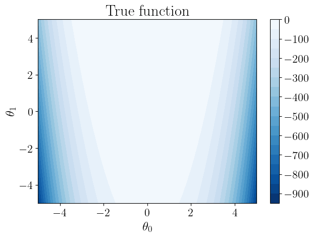
[7]:
sm.plot(plots=["true_fn_2D"])
Plotting true function contours 2D...
Saving to  results/rosenbrock_2d/true_function_2D.png
[7]:
[8]:
sm.plot(plots=["gp_fit_2D"])
Plotting gp fit 2D...
[8]:
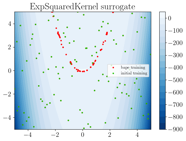
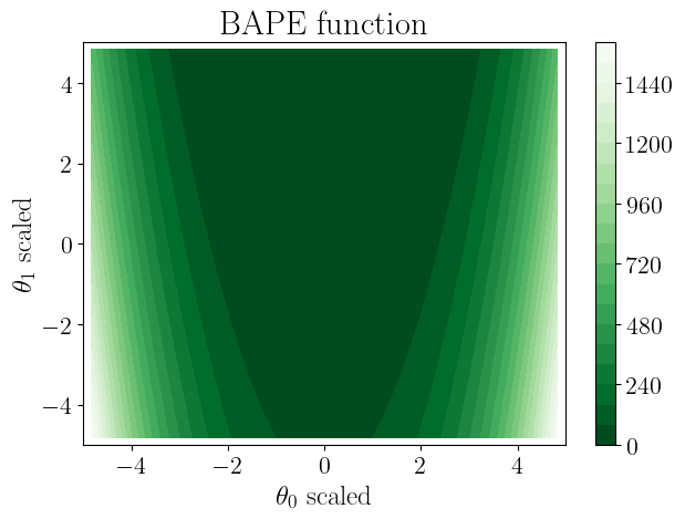
We can also check how the active learning function looks at this iteration. If the model is closed to converged, we expect the high probability regions to be close to 0.
[9]:
sm.plot(plots=["obj_fn_2D"])
Plotting objective function contours 2D...
Saving to  results/rosenbrock_2d/objective_function.png
[9]:
alabi also tracks various performance metrics as a function of active learning iteration. These results can be accessed from the dictionary:
[10]:
sm.training_results.keys()
[10]:
dict_keys(['iteration', 'gp_hyperparameters', 'gp_hyperparameter_opt_iteration', 'gp_hyperparam_opt_time', 'training_mse', 'test_mse', 'training_scaled_mse', 'test_scaled_mse', 'gp_kl_divergence', 'gp_train_time', 'obj_fn_opt_time', 'acquisition_optimizer_niter'])
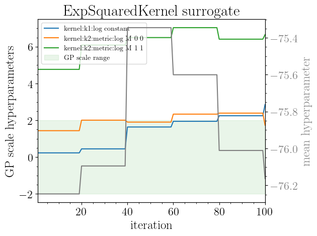
Here are some examples of quick plots you can make of these results:
[11]:
sm.plot(plots=["gp_hyperparameters"])
Plotting gp hyperparameters...
Saving to  results/rosenbrock_2d/gp_hyperparameters_vs_iteration.png
[11]:
[12]:
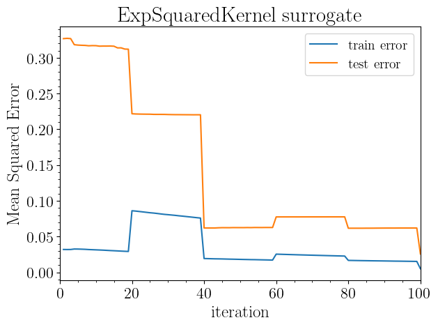
sm.plot(plots=["test_mse"])
Plotting the gp mean squared error with 1000 test samples...
Saving to results/rosenbrock_2d/gp_mse_vs_iteration.png
[12]:
[13]:
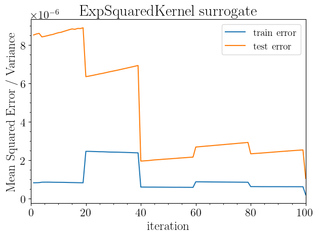
sm.plot(plots=["test_scaled_mse"])
Plotting the scaled gp mean squared error with 1000 test samples...
Saving to results/rosenbrock_2d/gp_scaled_mse_vs_iteration.png
[13]:
[ ]: